
Arguably the most important stage in selecting a cross-device identity graph provider is evaluation. More specifically: how does one compare cross-device matching solutions? Since there are no current industry standards or guidelines, this task can prove to be rather confusing and daunting! So in response, we at Roqad have compiled a thorough guideline to help you better understand how to test cross-device matching solutions and evaluate the quality of an identity graph.
1. Identity Graphs Building Blocks
To preface, an identity graph (IG) consists of vertices and undirected edges between some of the vertices. A vertex corresponds to a device (or more precisely to a device ID), such as a mobile device, desktop PC, tablet, etc. Each edge indicates whether there is a connection between two devices, (i.e., they belong to the same user). In the identity graph, devices belonging to the same user create a clique, (i.e., a fully-connected subgraph) In other words, a clique corresponds to a (anonymized) user.
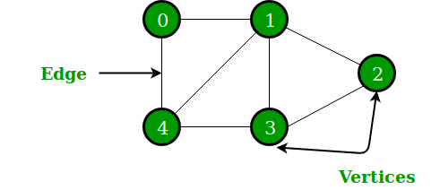
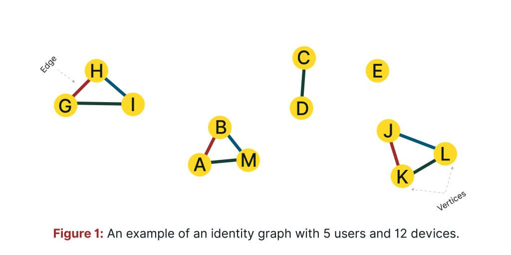
Let us illustrate! Fig. 1 shows an identity graph, in which there are 12 devices displayed. We’ve identified 5 cliques of devices (i.e., users). One clique has only 1 device, (E), another has 2 devices, (C, D), and the three remaining have 3 devices, (A, B, M), (H, G, I) and (J, K, L).
A device ID can be either a cookie, IDFA (Apple’s Identifier for Advertisers) or AAID (Android Advertising ID). A cookie identifies, for example, a desktop or a mobile web, while IDFA and AAID identify mobile devices.
2. Evaluation of Identity Graphs
There are two ways to test cross-device matching solutions:
- Supervised
- Unsupervised
The former can always be used even without any test data, and its main purpose is to check the overall structure of the graph. The latter requires a separate set of so-called deterministic data from which the true connections between devices are to be extracted.
2.1 Unsupervised Metrics
Typically, when using a cross-device matching solution, you would query an identity graph with a set of device IDs (e.g., provided by a client or partner). As an output you would obtain a subgraph consisting of all cliques, which contain at least one device ID from the query. This process is visualized in Fig. 2. The initial identity graph query contains a total of 6 devices:
A, B, C, D, E, and F. By applying the cross-device identity graph logic, you would get a subgraph with 3 cliques (clique in the graph theory sense, not mouse “clicks”… just checking if you’re paying attention)
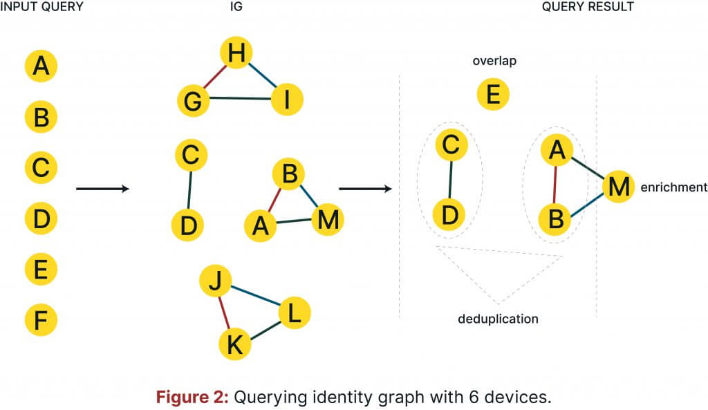
- Note that device F is missing in the response, which means that this device hasn’t been found within the graph.
- Device E has no connection to any other devices.
- Devices C and D belong to one user and form a clique
- Devices A and B belong to the same user who also owns device M.
Based on this output, you are able to compute several metrics. Overlap, which describes how many devices from the query are found in the graph, can be expressed by a fraction of overlapped devices to all devices included in the query. For this example, the overlap is ⅚ (i.e., five device IDs are also contained in the identity graph).
Once satisfied with the overlap, you can then check the number of device IDs from the query that are connected to each other (i.e., shared by the same user). This process is known as deduplication. It is expressed as a fraction of deduplicated devices to all device IDs included in the query. From the same example, the deduplication rate would be 4/6 since the following connections (A, B), (C, D) were identified and contain in total four devices from the query.
You can also measure whether other device IDs already exist in the graph, which are then connected to the devices from a query. These devices already found in the graph then enrich the input set. This metric is known as enrichment and can be expressed as a fraction of enriched device IDs to all device IDs included in the query. In our example, it would be 2/6 since only two devices from the query are connected to a new device (i.e., A and B are connected to M).
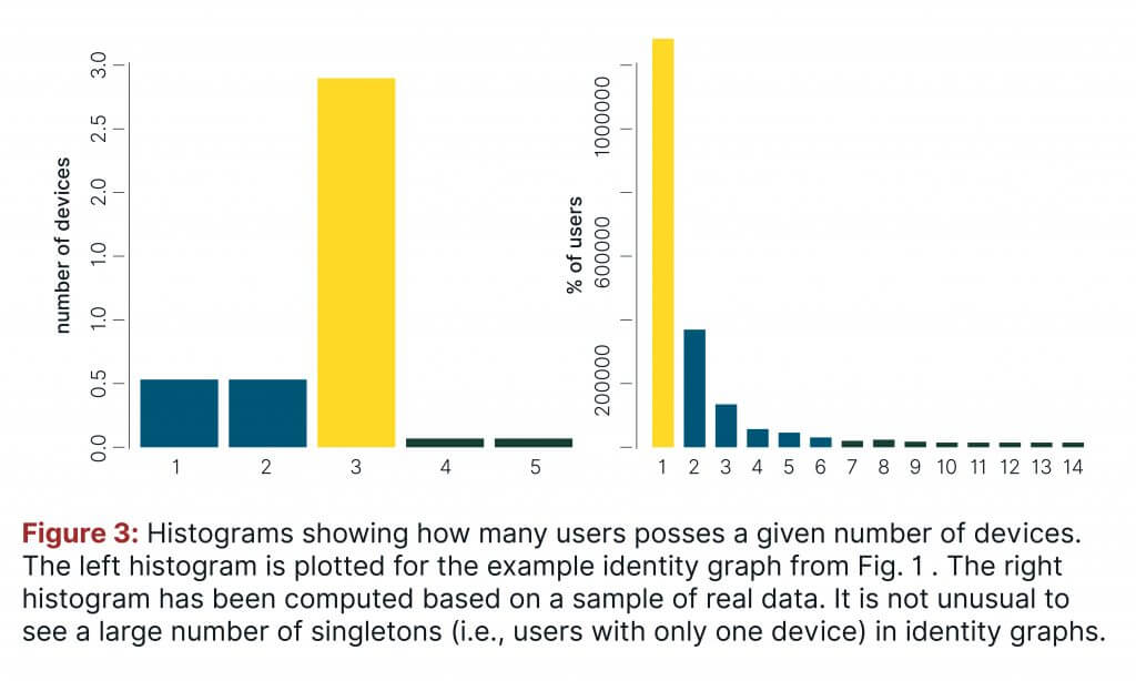
You are also able to derive other insights from the identity graph, such as statistics focusing on the number of users and/or devices found in the graph, as well as the number of connections between different types of devices (e.g., mobile-desktop). A histogram of the number of users with a given number of devices can also be easily obtained. These additional statistics further depict the structure of the graph. Keeping with the same example, the relevant histogram is visualised in the left plot of Fig. 3.
For real-life cases of utilizing real data within an identity graph, it is not unusual to see a large number of singletons (i.e., users with only one device). Additionally, some cliques can also be extremely large. In a well-designed identity graph, the number of devices per user should range from 2 to 15, and the number of users with 2 or 3 devices should be the largest. The right plot of Fig. 3 shows an exemplary histogram obtained on real data.
Ideally, each clique in the graph should contain different types of devices, as often found in the real world. There is also a common assumption that each individual user has access to one or two mobile devices as well as a desktop computer. Therefore, the number of mobile-mobile, mobile-desktop, or desktop-desktop connections in a graph can be an additionally intuitive metric used to depict the structure of an identity graph. In specific cases where a clique contains multiple desktop IDs only, you can suspect that the graph has deduplicated different IDs coming from one desktop device.
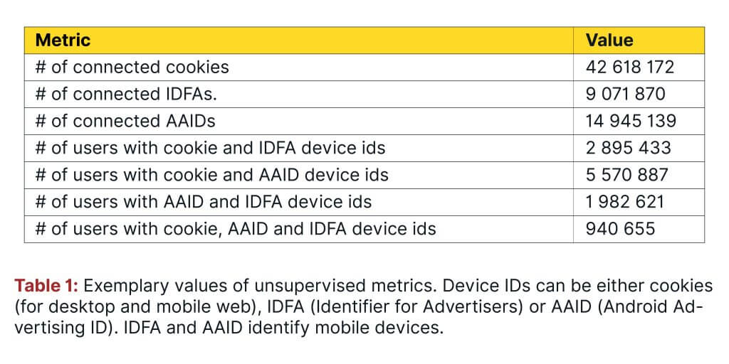
Table 1 shows exemplary numbers of different types of connections in the identity graph.
2.2 Supervised Metrics
In the previous subsection, you may have noticed that predictive performance of an identity graph was not mentioned. To be able to measure this form of performance, you would need to have a separate test set of deterministic data from which you could then extract true connections between devices.
Since obtaining ground truth data is usually difficult, your cross-device identity graph provider should be able to run the test using its data. In this specific case, you need to ensure that the users and their devices used for the test have not been touched while training the machine learning algorithms. Otherwise, the results obtained will reflect an overly optimistic output than what you would experience in reality; therefore, it is essential that the same data should not be used for both training and testing purposes. At Roqad, we ensure that these experiments are performed with 100% transparency.
(Ahem!)
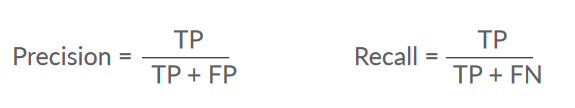
The predictive performance of identity graphs can be measured in terms of precision and recall.
Precision is a fraction of predicted matches between devices that are the actual/true ones, whereas recall is the fraction of total actual matches that are correctly identified. Precision and recall can be explained visually in Fig. 4, where true connections are the actual ones, and the positive connections are those that are predicted as positive by an identity graph.
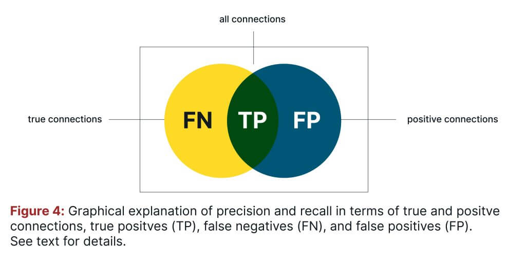
The intersection of true and positive connections are called true positives (TP). False negatives (FN) are the true connections that are not predicted as positive, and false positives (FP) are positive connections that are not true connections. Mathematically, precision and recall are defined as:
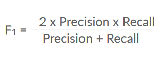
Achieving the ideal balance between precision and recall is one of the main goals of device matching.
This balance can be obtained by a harmonic mean of these two metrics and the result is often referred to as an F1 score:
To compute the performance metrics mentioned, you need to have a list of ground truth connections (GTC) obtained from deterministic data and a list of connections from an identity graph (IGC). In both lists you will use only those devices that are in the intersection of deterministic data and the IG. For instance, let us use the same IG as before, containing devices A, B, M, C, D, E, H, G, I, J, K, and L.
Let us also assume that the following devices are included in the deterministic data: A, B, C, D, E, F, G, X, and Y. Fig. 5 recalls the structure of the identity graph and presents the graph based on connections from deterministic data. The intersection of both lists of devices is: A, B, C, D, E, and G.
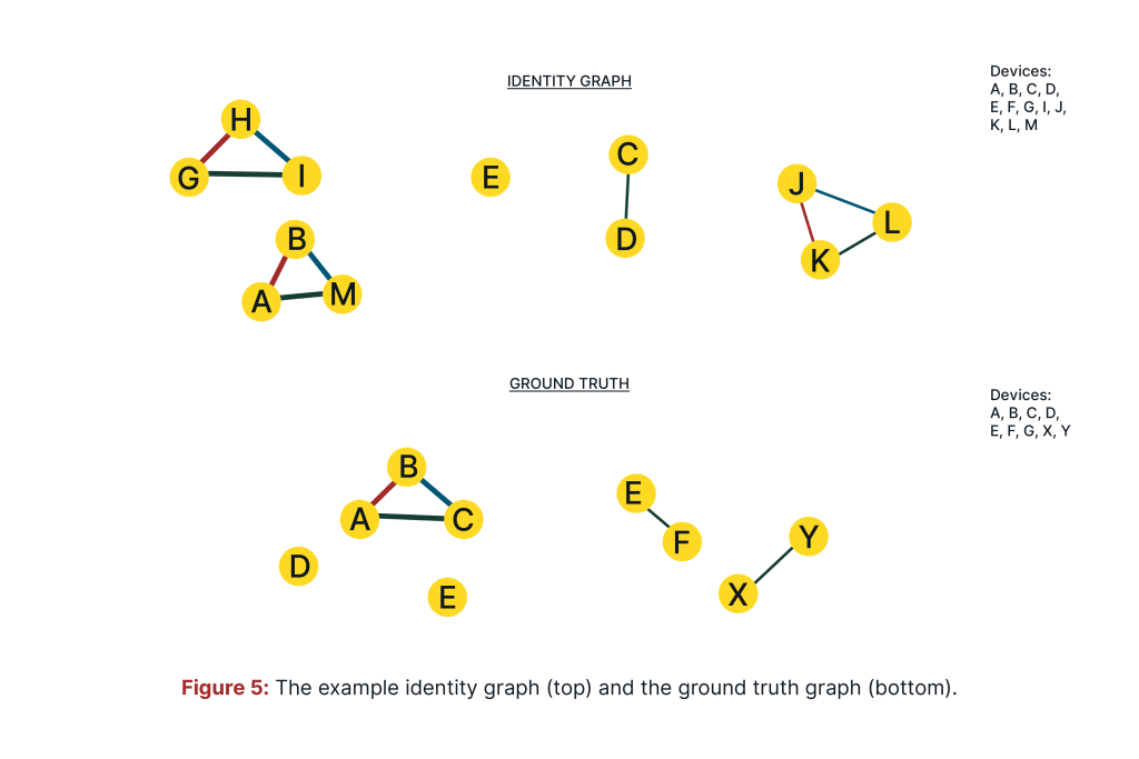
The GTC list contains four connections extracted from the deterministic data and the IGC list has two connections. These connections are listed in Table 2. To avoid duplicates in the lists (e.g., “A, B” and “B, A”) we assume a lexicographic order of device IDs in each connection.
You need to remember, however, that you should not expect the ground truth connections to be a perfect reflection of the real world, since this information is also obtained from logs. Therefore, we might not see all connections between devices and observe many singleton users (in the example, we have two such users).
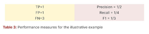
By using the lists above, the computation of precision, recall, and the F1 score is straightforward. Thereby you can compute TP, FP, and FN by using set operations (we use ∩ to denote set intersection and \ for set difference):
TP = GTC ∩ IGC
FP = IGC \ GTC
FN = GTC \ IGC
Table 3 provides the values of performance measures for our example.
Please note, however, that one needs to be very careful in comparing the values of these measures obtained on different test sets. This is due to the fact that precision decreases as the number of users included in a test set increases. This is because the number of possible connections increases quadratically with the number of users. The same concerns the number of FP. In turn, TP and FN grow linearly with the number of users, therefore recall is much more stable as it is computed solely on TP and FN. It should be constant for different numbers of users in the test set.
Fig. 6 shows the empirical results of precision and recall obtained on a test set with a varying number of users.
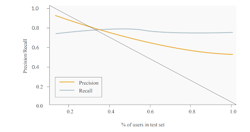
Figure 6: Precision and recall for a test set with a different number of users. The x axis shows the percentage of users used for computing precision and recall.
Based on the above discussion, a natural question arises: what are the right metrics for testing predictive performance of an identity graph? Precision and recall seem to have become a standard, but the shortcomings of precision are not often discussed. Of course machine learning offers plenty of performance measures that are regularly used for testing predictive models. Unfortunately, many of them are not useful in testing cross-device identity graphs.
For example, accuracy and AUC (i.e., area under the ROC curve) strongly depend on true negatives (TN), or “no connections’ between devices that are also predicted as “no connections’ ‘ (i.e., as negatives). Since there are much more unconnected pairs of devices than the connected ones (the number of ‘no connections’ grows quadratically with the number of devices), and the true connections are actually the ones we care about, it would be very confusing and misleading to use these types of metrics. For example, accuracy is defined as a fraction of TP and TN to all possible connections. Since TN will dominate all other quantities, accuracy will always be very close to 1.
Let us finalize this section by underlining that there is still room for new metrics and methodologies for testing performance of identity graphs. Roqad works intensively on delivering the right methodology for this purpose.
3 Final Thoughts
You are now equipped with the basic measurement tools to help you evaluate a cross-device identity graph’s performance using unsupervised and supervised metrics. It is important to remember that testing cross-device identity graphs is in general quite tricky since the number of possible connections between devices grows quadratically with the number of devices in the test set. Therefore, it is not easy to compare results obtained on different data sets.
Stay in the Know
Get news, resources and updates about events happening in the world of digital advertising.